Chapitre 4 Profiler son code

On parle de profiling en anglais. Il s’agit de déterminer ce qui prend du temps dans un code. Le but étant, une fois trouvé le bloc de code qui prend le plus de temps dans l’exécution, d’optimiser uniquement cette brique.

Pour obtenir un profiling du code ci-dessous, sélectionner les lignes de code d’intérêt et aller dans le menu “Profile” puis “Profile Selected Lines”. Cela utilise en fait la fonction profvis() du package profvis.

n <- 10e4
pdfval <- mvnpdf(x=matrix(1.96, nrow = 2, ncol = n), Log=FALSE)

Flame Graph

Data

Options ▾

mypkgr/R/mvnpdf.R		Memory				Time
	#' Multivariate-Normal probability density function
	#'
	#' This is a concise description of what the function does.
	#'
	#' This part gives more details on the function.
	#'
	#' @param x a p x n data matrix with n the number of observations and
	#'p the number of dimensions
	#' @param mean mean vector
	#' @param varcovM variance-covariance matrix
	#' @param Log logical flag for returning the log of the probability density
	#'function. Default is \code{TRUE}.
	#'
	#' @return a list containing the input matrix x and y the multivariate-Normal probability density function
	#' computed at x
	#'
	#' @export
	#'
	#' @examples
	#' mvnpdf(x=matrix(1.96), Log=FALSE)
	#'dnorm(1.96)
	#'
	#'mvnpdf(x=matrix(rep(1.96, 2), nrow=2, ncol=1), Log=FALSE)
	mvnpdf <- function(x, mean = rep(0, nrow(x)),
	varcovM = diag(nrow(x)), Log = TRUE) {
	n <- ncol(x)
	p <- nrow(x)
	x0 <- x - mean
	Rinv <- solve(varcovM)
	LogDetvarcovM <- log(det(varcovM))
	y <- NULL
	for (j in 1:n) {
	yj <- - p/2 * log(2*pi) - 0.5 * LogDetvarcovM -
	0.5 * t(x0[, j]) %*% Rinv %*% x0[, j]
	y <- c(y, yj)
	}
	if (!Log) {
	y <- exp(y)
	}
	res <- list(x = x, y = y)
	class(res) <- "mvnpdf"
	return(res)
	}
	#' Plot of the mvnpdf function on the first dimension
	#'
	#' @param x an object of class \code{mvnpdf} resulting from a call of
	#' \code{mnvpdf()} function.
	#' @param ... graphical parameters passed to \code{plot()} function.
	#'
	#' @return Nothing is returned, only a plot is given.
	#' @export
	#' @importFrom graphics plot
	#' @examples
	#' pdfvalues <- mvnpdf(x=matrix(seq(-3, 3, by = 0.1), nrow = 1), Log=FALSE)
	#' plot(pdfvalues)
	plot.mvnpdf <- function(x, ...) {
	graphics::plot(x$x[1, ], x$y, type = "l", ylab="mvnpdf", xlab="Obs (1st dim)", ...)
	}

Sample Interval: 10ms

14810ms

☒ Split horizontally

☒ Hide internal function calls

☐ Hide lines of code with zero time

☐ Hide memory results

OK, we get it ! Concaténer un vecteur au fur et à mesure dans une boucle n’est vraiment pas une bonne idée.

4.1 Comparaison avec une version plus habile de mnvpdf()

Considérons une nouvelle version de mvnpdf(), appelée mvnpdfsmart(). Télécharger le fichier puis l’inclure dans votre package.

Profiler la commande suivante :

n <- 10e4
pdfval <- mvnpdfsmart(x=matrix(1.96, nrow = 2, ncol = n), Log=FALSE)

Flame Graph

Data

Options ▾

mypkgr/R/mvnpdfsmart.R		Memory				Time
	#' @rdname mvnpdf
	#' @export
	mvnpdfsmart <- function(x, mean = rep(0, nrow(x)),
	varcovM = diag(nrow(x)), Log = TRUE) {
	n <- ncol(x)
	p <- nrow(x)
	x0 <- x - mean
	Rinv <- solve(varcovM)
	LogDetvarcovM <- log(det(varcovM))
	y <- rep(NA, n)
	for (j in 1:n) {
	yj <- - p/2 * log(2*pi) - 0.5 * LogDetvarcovM -
	0.5 * t(x0[, j]) %*% Rinv %*% x0[, j]
	y[j] <- yj
	}
	if (!Log) {
	y <- exp(y)
	}
	res <- list(x = x, y = y)
	class(res) <- "mvnpdf"
	return(res)
	}

Sample Interval: 10ms

210ms

☒ Split horizontally

☒ Hide internal function calls

☐ Hide lines of code with zero time

☐ Hide memory results

On a effectivement résolu le problème et on apprend maintenant de manière plus fine ce qui prend du temps dans notre fonction.

Pour confirmer que mvnpdfsmart() est effectivement bien plus rapide que mvnpdf() on peut re-faire une comparaison avec microbenchmark() :

n <- 1000
mb <- microbenchmark(mvnpdf(x=matrix(1.96, nrow = 2, ncol = n), Log=FALSE),
                     mvnpdfsmart(x=matrix(1.96, nrow = 2, ncol = n), Log=FALSE),
                     times=100L)
mb

## Unit: milliseconds
##                                                            expr      min
##       mvnpdf(x = matrix(1.96, nrow = 2, ncol = n), Log = FALSE) 3.138591
##  mvnpdfsmart(x = matrix(1.96, nrow = 2, ncol = n), Log = FALSE) 2.330481
##        lq     mean   median       uq      max neval cld
##  3.322681 3.778820 3.437030 3.580571 8.138008   100  a 
##  2.360309 2.447065 2.381362 2.425847 6.387636   100   b

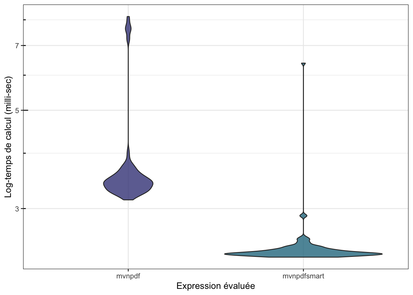
Et on peut également voir si on devient compétitif avec dmvnorm() :

n <- 1000
mb <- microbenchmark(mvtnorm::dmvnorm(matrix(1.96, nrow = n, ncol = 2)),
                     mvnpdf(x=matrix(1.96, nrow = 2, ncol = n), Log=FALSE),
                     mvnpdfsmart(x=matrix(1.96, nrow = 2, ncol = n), Log=FALSE),
                     times=100L)
mb

## Unit: microseconds
##                                                            expr      min
##              mvtnorm::dmvnorm(matrix(1.96, nrow = n, ncol = 2))   43.747
##       mvnpdf(x = matrix(1.96, nrow = 2, ncol = n), Log = FALSE) 3147.857
##  mvnpdfsmart(x = matrix(1.96, nrow = 2, ncol = n), Log = FALSE) 2308.546
##         lq       mean   median       uq       max neval cld
##    51.8445   73.05421   74.251   89.749   117.424   100 a  
##  3295.1085 3715.51266 3416.387 3522.740  8054.737   100  b 
##  2348.0085 2504.66540 2379.497 2428.163 10087.189   100   c

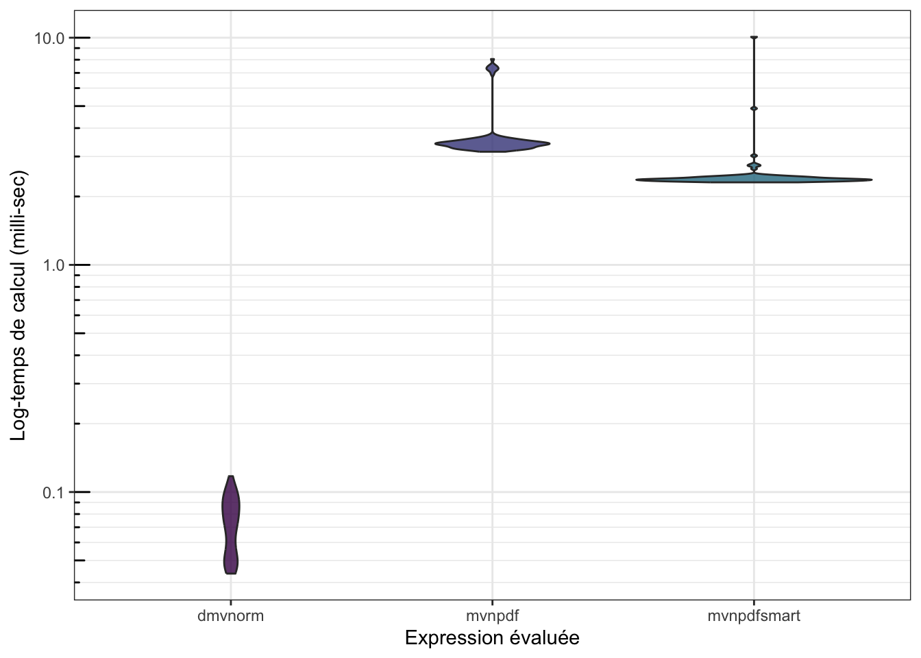
Il y a encore du travail…

4.2 Comparaison avec une version optimisée dans

Boris est arrivé, après de longues recherches et plusieurs tests, à une version optimisée avec les outils de .

Inclure la fonction mvnpdfoptim() dans le package, puis profiler cette fonction :

n <- 10e4
profvis::profvis(mvnpdfoptim(x=matrix(1.96, nrow = 2, ncol = n), Log=FALSE))

Flame Graph

Data

Options ▾

mypkgr/R/mvnpdfoptim.R		Memory				Time
	#' @rdname mvnpdf
	#' @export
	mvnpdfoptim <- function(x, mean = rep(0, nrow(x)),
	varcovM = diag(nrow(x)), Log=TRUE){
	if(!is.matrix(x)){
	x <- matrix(x, ncol=1)
	}
	n <- ncol(x)
	p <- nrow(x)
	x0 <- x-mean
	Rinv <- backsolve(chol(varcovM), x=diag(p))
	xRinv <- apply(X=x0, MARGIN=2, FUN=crossprod, y=Rinv)
	logSqrtDetvarcovM <- sum(log(diag(Rinv)))
	quadform <- apply(X=xRinv, MARGIN=2, FUN=crossprod)
	y <- (-0.5*quadform + logSqrtDetvarcovM -p*log(2*pi)/2)
	if(!Log){
	y <- exp(y)
	}
	res <- list(x = x, y = y)
	class(res) <- "mvnpdf"
	return(res)
	}

Sample Interval: 10ms

190ms

☒ Split horizontally

☒ Hide internal function calls

☐ Hide lines of code with zero time

☐ Hide memory results

Et un petit microbenchmark() :

n <- 1000
mb <- microbenchmark(mvtnorm::dmvnorm(matrix(1.96, nrow = n, ncol = 2)),
                     mvnpdf(x=matrix(1.96, nrow = 2, ncol = n), Log=FALSE),
                     mvnpdfsmart(x=matrix(1.96, nrow = 2, ncol = n), Log=FALSE),
                     mvnpdfoptim(x=matrix(1.96, nrow = 2, ncol = n), Log=FALSE),
                     times=100L)
mb

## Unit: microseconds
##                                                            expr      min
##              mvtnorm::dmvnorm(matrix(1.96, nrow = n, ncol = 2))   43.337
##       mvnpdf(x = matrix(1.96, nrow = 2, ncol = n), Log = FALSE) 3154.499
##  mvnpdfsmart(x = matrix(1.96, nrow = 2, ncol = n), Log = FALSE) 2314.450
##  mvnpdfoptim(x = matrix(1.96, nrow = 2, ncol = n), Log = FALSE) 1747.871
##         lq       mean   median        uq      max neval  cld
##    53.6075   73.60197   75.235   90.3025  142.680   100 a   
##  3301.1970 3824.36479 3398.121 3571.4485 8685.276   100  b  
##  2368.7135 2419.81877 2401.309 2434.4365 3397.875   100   c 
##  1794.3855 1922.38012 1828.580 1863.3475 6635.522   100    d

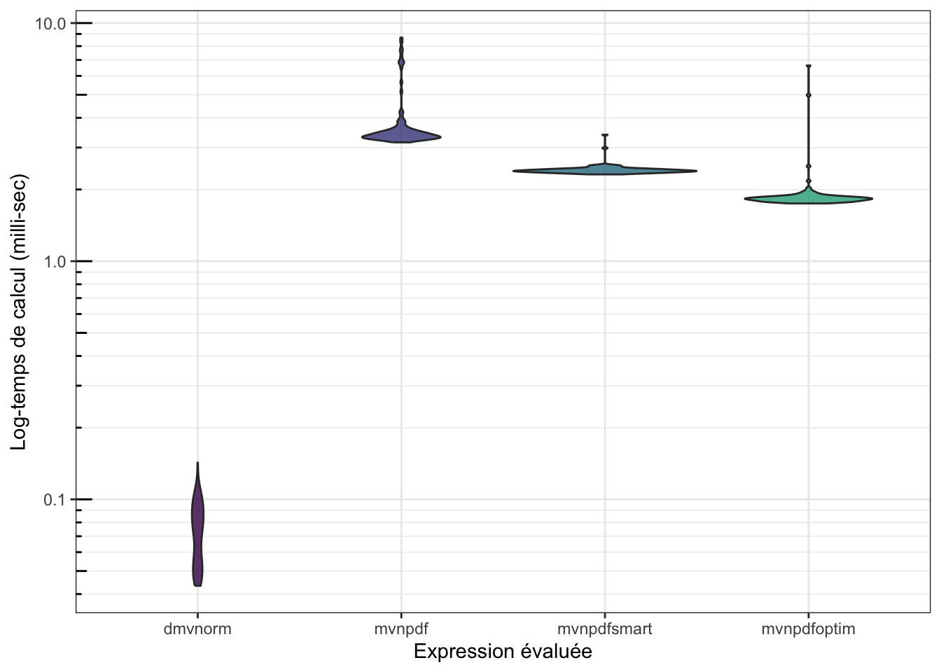
Pour finir on peut profiler la fonction dmvnorm() :

n <- 10e5
library(mvtnorm)
profvis::profvis(dmvnorm(matrix(1.96, nrow = n, ncol = 2)))

Flame Graph

Data

Options ▾

(Sources not available)

Sample Interval: 10ms

100ms

☒ Split horizontally

☒ Hide internal function calls

☐ Hide lines of code with zero time

☐ Hide memory results